MS EXCEL - Introduction

Page 1

A spreadsheet is essentially a matrix of rows and columns. Consider a sheet of paper on which horizontal and vertical lines are drawn to yield a rectangular grid. The grid namely a cell is the result of the intersection of a row with a column. Such a structure is called a

Spreadsheet.

A spreadsheet package contains an electronic equivalent of a pen, an eraser, and a large sheet of paper with vertical and horizontal lines to give rows and columns. The cursor position uniquely shown in dark mode indicates where the pen is currently pointing. We can enter text or numbers at any position on the worksheet. We can enter a formula

in a cell where we want to perform a calculation and the results are to be displayed. A powerful recalculation facility jumps into action each time we update the cell contents with new data.

MS Excel is the most powerful spreadsheet package brought by Microsoft. The three main components of this package are Electronic spreadsheet Database management Generation of Charts. 

Each workbook provides 3 worksheets with the facility to increase the number of sheets. Each sheet provides 256 columns and 65536 rows to work with. Though the spreadsheet packages were originally designed for accountants, they have become popular with almost

everyone working with figures. Sales executives, book-keepers, officers, students, research scholars, investors bankers, etc, almost anyone find some form of application for it.

You will learn the following features at the end of this section. Starting Excel 2003 Using Help Workbook Management Cursor Management Manipulating Data Using Formulae and Functions Formatting Spreadsheet Printing and Layout Creating Charts and Graphs

Page 2

Starting Excel 2003 Switch on your computer and click on the Start button at the bottom left of the screen. Move the mouse pointer to Programs, then across to Microsoft Excel, then click on Excel as shown in this screen.

When you open Excel a screen similar to this will appear

The options shown below are called Menu Bar

The collection of icons for common operations shown below is called as Standard Tool Bar

The formula bar is the place in which you enter the formula(=A3*B5)

The alphabets A, B… are known as columns

This is the name of the workbook. (Book1)

The rows are numbered as 1,2,3…

Sheet1, Sheet2, and Sheet3 are known as worksheet tabs

How to use the Help Menu

Click on Help, Contents, and Index, then click on the Index tab. The following screen will appear

Type the first few letters to see the help entries for those letters. You can get the printout of any help topic by selecting it, right-clicking, and then clicking Print Topic.

Workbook Management Task 1: Creating a new workbook Click on the File menu and then click on New.

Click Workbook and then click the OK button. You will get the screen as shown below.

Enter data as shown in the figure below :

Task 2: Saving Workbook

Click on the File menu and then click Save. You will get the below screen

In the File name text box, type sample and then click the Save button

Task 3: Opening an existing workbook

Click on the File menu and click on Open. The open dialog box will appear

Click on some file (Example: sample.xls), then click on Open. Task 4: Closing your workbook Click on the File menu, then click Close to close your workbook Cursor Management

Task 1: Moving around the worksheet Open sample.xls workbook. Move the cursor in your worksheet by using the arrow keys on the right-hand side of the keyboard. When you have got lots of rows of data you can move the cursor more quickly by using the PgUp and PgDn keys to move up and down a screen at a time. To move one screen to the right, press the Alt key and PgDn keys together. To move one screen to the left, press the Alt and PgUp keys together. To move further to the right, just keep pressing the right arrow key to move back to cell A1, and press the Ctrl and Home keys together. Pressing the Home key on its own takes you back to column A To move to the last column(IV) press the Ctrl and right arrow keys together. MS Excel Page 11 of 40 To move to the last cell containing data, press Ctrl and End keys together. To move to the last row(65,536), press Ctrl and the down arrow keys together. You can also move the cursor with the mouse. Move the mouse

pointer to the location you want. Press and release the left mouse button once when the cursor is where you want it. Task 2: Moving to a Specified cell Click on the Edit menu, and choose Go To. You will get the below screen

Enter the destination cell reference in the Reference text box. Click OK to move directly to the specified cell. Data Manipulation

Task 1: Entering data

Start Excel. Click File and then New. An empty worksheet appears as shown below

Type Expenditure in cell A1 then presses down the arrow key to move to cell A2.

Type Month then press the down arrow key to move to cell A3 Continue to type the data. The resulting worksheet should appear on the following screen.

Save your work by clicking File and then Save As. This dialog box appears.

Type cash in the File Name text box and then click the Save button. Excel automatically adds the extension .xls to your file name.

Task 2: Editing data

Click File and then click Open.

Click cash.xls and then click Open.

Move the mouse pointer to cell D4, click and release. The cell is highlighted and 18 appears in the formula bar.

Move the mouse pointer to the formula bar and click once to the right of 18.

Use the Backspace key to delete 8, then type 4 and press Enter. Cell D4 now contains the value 14. 

Task 3: Replacing cell data

Make cell B5 active by clicking on it. Type 200 and press Enter. Cell B5 will now contain the value 200 replacing the old value (150). 

Task 4: Deleting cell contents

Move to cell C5 and click to select. Press the Delete key. The cell becomes blank. Drop down the Edit menu and click Undo to reinstate the 145. Excel 97 allows 16 levels of undoing. You can use Undo and Redo buttons also.

Task 5: Copying data

Open the cash spreadsheet. Select the cells D3 to D5 Click the Edit menu and then click Copy.

Select the cells F3 to F5. Click the Edit menu and then click Paste. Now the cells D3 to D5 are copied into F3 to F5. 

Task 6: Moving data

Open cash.xls spreadsheet. Select the cells from B3 to B5. Click the Edit menu and then click Cut. Select cells G3 to G5. Click the Edit menu and then click Paste. 

Task 7: Data AutoFill

There is an easy method to fill the data in columns and rows. The data may be Numeric or dates and text. To fill Sono by using autofill ¨ Type Sono for 2 cells i.e 1,2 in the cells A1 and A2 respectively. ¨ Select two cells and drag the Fill Handle + To fill dates in the cells

¨ Type the date in the cell ¨ Select the cell and drag the Fill Handle We can customize the lists with different text data to minimize the redundancy of work. Some of the lists are listed below:

1. Jan, Feb, Mar, Apr, May, June, July…. like months

2. Sunday, Monday, Tuesday, Wednesday, Thursday…Like weekdays

3. Adilabad, Anantapur, Chittor, Cuddapah… like District names

4. Ravi, Kiran, Praveen, Rama…. like employees list

To create a customized list follow the steps given below:

¨ Click Tools Menu, Click Options then click Custom Lists tab, Then you will find the figure given below:

Click NEW LIST and enter the list in the List entries window ¨ Click Add button then click on the OK button then your list will be added to the Custom Lists. That list you can use as and when required to type.

¨ Now you can drag the fill handle (+ ) to get the list automatically. Using Formulae and Functions

Task 1: Entering a formulae

Click File and then click New. Enter the data in the new worksheet as shown below

Cell B6 should contain a formula. Move the cell pointer to cell B6. Type =B3+B5(formulae and functions should always begin with = sign) Cell B6 will now contain the value 350 Look at cell B6; you will see the result of the formula in cell B6 rather than the formula. Now repeat the appropriate formula for cells C6 and D6. Save your worksheet as cash3.xls. 

Task 2: Editing Formulae

Move the cursor to the formula bar with the mouse, clicking once. Make the desired changes. When you have finished editing the formulae, press the Enter key for the changes to take effect. (OR) Edit the contents by pressing the F2 key on the keyboard 

Task 3: Displaying and Printing formulae

Click the Tools menu and then click Options. Click the View tab. In Window, options check the Formulas checkbox. The below screen appears.

Click the OK button.

To print the worksheet with formulae displayed, click the File menu and click on Print Preview. If the layout is satisfactory, click on the Print button.

Task 4: Using the SUM function

Open cash3.xls spreadsheet.

Suppose you want the summation of the cells B3 to B5 should appear in cell B6, then first select the cells from B3 to B6. Click the Auto Sum icon on the toolbar. The result of (B3+B4+B5) will appear in cell B6.

Task 4: Copying Formulae

Open cash3.xls spreadsheet.

If you want to copy the formula in cell B6 to C6, D6, and E6 then first select cell B6. Move the cursor to the lower right corner of cell B6. The cursor will change to the + icon. Drag the cursor from B6 to E6 and release the left mouse button. You will notice that the cells C6, D6, and E6 are updated immediately as shown below.

Task 5: Copying formulae using absolute addressing

Create the worksheet shown below and save ABS If you copy the formula in the cell c2 to c3, c4, and c5 you will get the incorrect result because the formula will change in the cell (C3)to B3*A10 but the value in the A10 is not defined. The reason is that we are copying the relative address but not the absolute address. To use absolute address move to the c2 cell. Edit the formula to =B2+($B$2*$A$9) and press Enter key. Copy the formula to cells C3 to C5.

Task1: Increasing column width

Open an existing worksheet(For example cash3.xls)

Move the mouse pointer to the position(column B)shown below in the column header. When the black cross appears, hold down the left button and drag the mouse to the right to increase the column width by the required amount.

Task 2: Decreasing column width

Open cash3.xls spreadsheet.

Move the mouse pointer to column B. When the black cross appears, hold down the left button and drag the mouse to the left to reduce the cell width.

Task 3: Changing the width of all cells in a spreadsheet

Open cash3.xls spreadsheet

Select the entire worksheet by clicking the Select All button (to the left of the A1 cell) at the top left corner of the worksheet. The worksheet changes from white to black.

Click the Format menu, click Column, then click Width In the column width text box type 20, then click the OK button. Your worksheet cells should all increase in width. You will get the below screen. You will notice that the widths of all columns are now changed to 20

Click the Undo button to revert to the previous cell width. 

Task 3: Inserting Columns

Open cash.xls spreadsheet.

Move to cell B2 and click. Click Insert menu, and click Columns. You will get the below screen. A blank column will be inserted before(to the left of column B)

Task 4: Deleting Column contents

Open cash.xls spreadsheet.

Move the mouse pointer to the column E header and click to select

column E

Press the Delete button. The column contents will be deleted. Click Undo button to revert to the previous screen.

Task 5: Removing columns, rows, and cells completely

Select individual columns or rows or cells. Click the Edit menu and click Delete

Task 5: Removing columns, rows, and cells completely

Select individual columns or rows or cells. Click the Edit menu and click Delete

Task 6: Inserting a row

When you insert a row, it is inserted above the current row, so if you want to insert a new row above row 6(between rows 5 and 6), place the cursor on a cell in row 6 and Click on the Insert menu. Click Entire Rows and insert a blank row between rows 5 and 6.

Task 7: Deleting row contents

Open cash.xls spreadsheet.

Move the mouse pointer to the row 2 header and click to select the row as shown below Press Delete to remove the contents of the row. Click the Undo button to cancel the delete operation.

Task 7: Inserting cells

Open cash.xls spreadsheet.

Select cells B2 to D4 by moving the mouse pointer to cell B2, holding down the left mouse button and dragging the mouse pointer to cell D4, then releasing the left button. The cells should be highlighted. Click the Insert menu and click Cells. This dialog box appears. Click OK to shift the cell down.

Task 8: Changing data justification

Open cash.xls spreadsheet.

Select cell B2 as shown below. Here the text “Jan” by default left-justified. You can modify alignment as right justified or center by clicking right-justify or center the text within the cell by clicking respectively. 

Task 9: Merge and Center data

Open cash.xls spreadsheet.

Select the cells A1 to H1 as shown below Create a new spreadsheet as shown below and save it as “marks.xls” Now you can format the cells in column C by selecting column C by clicking on the column heading

Click the Format menu and click on Cells. Click on Number. Use the Down arrow in the Decimal Places to set it to 0. Click OK. Now repeat the formatting but this time format the cells to two decimal places. Again, repeating the formatting operation, but this time to four decimal places. Finally, format the cells to eight decimal places. This screen will appear. The #### symbols indicate that the cell is too narrow to display the data in the chosen format. However, if you increase the cell width sufficiently, the data will be displayed in eight decimal places.

Increase the width of column C until the data is displayed. Now change the formatting back to two decimal places, and reduce the column width to a suitable width. Changing the data Orientation (Vertical, Horizontal, etc.) Excel offers three options that let you control the orientation of the text within a cell. These are Text alignment, Text orientation,

and Text control.

Vertical text alignment can be any one of the following

¨ Choose Cells from the Format menu.

¨ Click the Alignment Tab.

¨ Specify the desired text orientation by selecting one of the orientation boxes.

¨ Select the Wrap text check box if you want Excel to wrap the text ¨ Click OK

Here are some examples of the different alignment options

Printing and layout

Task 1: Previewing a printout

Open cash.xls spreadsheet.

Click on the File menu and click on Print Preview. A screen similar to this should appear. button, it magnifies the worksheet. Clicking on Zoom a second time returns you to the original preview format. Press PgDn to move through your worksheet if it is more than

one page long. Before printing makes sure that your printer is switched on, is loaded with the appropriate paper, and is one-line. If you are happy with the layout of your document, click on the Print button to obtain a printout. You should see a message on the screen telling you that your file is being a printer, and on which paper.

Task 2: Printing Landscape

To select landscape mode, click on the File menu, Page Setup this screen will appear.

Click on the Landscape button.

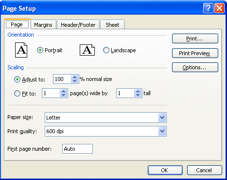
Task 3: Fitting your worksheet to one page

In the above screen click on the Fit To box and type: 1 page wide by 1 page tall. If you need to make changes to your worksheet before printing, click on the Close button to return to your workbook. 

Task 4: Adjusting margins

In the Page Setup dialog box, click the Margins tab and enter the appropriate sizes(in inches or centimeters) 

Task 5: Setting Header/Footer to your worksheet

From the Page Setup dialog box, click on the Header/Footer tab to display the below screen. In the Header box either select a title from the drop-down menu or enter your own title. Similarly for the Footer box also you can set your own title. Click on OK.

Task 6: Printing selected cells

Open cash.xls spreadsheet.

Click on the row 2 button (or any other row containing data) to highlight the entire row. Click on File, Print Area, and Set Print Area. The preview screen should only display the selected cells. (Row 2). If the preview is satisfactory, click the Print button to print out only row 2. Click on File, Print Area, and Clear Print Area to reset the Print Area.

Creating charts and graphs

Task 1: Creating a Pie Chart

Open cash.xls spreadsheet.

Select the cells A1 to G5 as shown below Click on the Insert menu and click the Chart option. This will start with the Office Assistant, guiding you through creating a chart. Follow the instructions in each step of the Wizard. The Assistant explains each step. In step 3, you can specify the Chart title, X-axis title, and Y-axis title separately. At step 4, click As an object in sheet 1, then click Finish. Your chart is now finished. Save as cash4. After that, Your chart is saved with the spreadsheet. This type of chart is known as an embedded chart and is saved with its worksheet.

Task 2: Creating charts when the data range is not continuous

Open cash4.xls

If your requirement is to create a chart to show expenditure for February, then first select cells A2 to A5. Hold down the Ctrl key and, while holding it down, select cells C2 to C5. Your screen should be similar to this one. Click on the Chart Wizard and create a column chart. Your screen should look similar to this. If your chart doesn’t appear to show any data, you probably included some other cells, probably A1 and/or C1. If so, delete your chart and re-select the correct range.

Task 3: Sizing a chart

¨ Open the cash3.xls created earlier. A screen similar to this one should appear. The small black markers are at each corner and mid-way along each side of the chart. These indicate that the chart is selected, and are called its selection squares. Click on the mid-point marker on the right-hand side, hold down the left mouse button and drag the mouse to the right about one inch(3cm), then release the mouse. The width of the chart will have increased. Now practice the same operation on the mid-point marker of each of the other sides of the chart. Now try the above, but this time on one of the four corner markers. Note that when you use these techniques, the whole chart changes in size, but it retains its original proportions. Now use the same technique to reduce the size of the chart. Task 4: Deleting Charts Make sure the chart is selected(the small black markers are visible). If not, move the mouse pointer into the chart area and click and release the left mouse button once. Press Delete to delete the chart.

Task 5: Moving charts and graphs

Make the chart active.

Move the mouse pointer into the chart area. Hold down the left mouse button and drag the chart to the desired position.

Task 6: Chart headings and labels

While creating charts step3 asks for Chart headings and labels for X-axis and Y-axis. You can define your own labels or click the Next button so that the default values can be accepted.

For example, the Chart title is Expenditure, the X-axis label is months and

The Y-axis label is the Sales

Task 7: Editing chart items

Create the chart as shown below and save it as cash4.xls. Click the chart title(Expenditure). Selection markers(small black squares) will appear around the selected item. You can move or size the title in the same way that you can move or size a chart. Click the title box and drag it up by about one inch (3 cm), then release the mouse. You can format the title by selecting it, then right-clicking, and then selecting “Format Chart Title” from the drop-down menu. You will get the below screen. You can select font type, font style, and font size as shown above Click OK.

Task 8: Adding text to a chart

Open cash3.xls worksheet.

Click the View menu, click Toolbars, and Drawing. Click the Text box icon on the Drawing toolbar.

Draw a text box inside the chart area as shown below Click inside the text box. A flashing text cursor will appear. Now type Household Expenditure You can use the same procedure for any other text that you want to appear in charts.

Task 9: Adding a legend to a chart

Create a pie chart as shown below.

Display the Chart toolbar, by dropping down the view menu and clicking Toolbars, Chart. In the above figure, the legend is already added. Click inside the pie chart, then click once on the add or delete legend button on the Chart toolbar. The legend will be added if not already present and removed if it is currently present. You can also add or delete a legend from the Chart, Chart options menu

Task 10: Adding gridlines to a chart

Open the cash3.xls worksheet and change the chart type to a Column chart. Click Chart, Chart options to display this box. Click the Gridlines tab and tick the gridlines boxes required.

Task 11: Adding data labels to a chart

Open the cash3 worksheet and change the chart type to the pie chart. Drop down the chart menu and click Chart options. Click on the Data Labels tab. Click on Show label and percent. Your screen should look similar to this.